Difference between revisions of "Learn Easy Java Simulation"
m (added Category:Explore an application using HotCat) |
|||
| Line 25: | Line 25: | ||
{| class="wikitable" | {| class="wikitable" | ||
|- | |- | ||
| − | |style="width: 50%;| | + | |style="width: 50%;|[[File:Easy_Java_Simulation_1_EXAMPLE.jpg|450px]] |
| − | |style="width: 50%;| | + | |style="width: 50%;|[[File:Easy_Java_Simulation_2_Model_Variables.jpg|450px]] |
|- | |- | ||
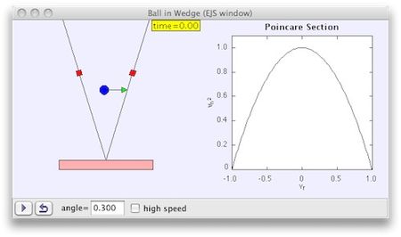
|style="width: 50%;|Step 1- The image is a screenshot of an EJS simulation modeling the path of a ball confined to move between two walls that form a wedge shape. | |style="width: 50%;|Step 1- The image is a screenshot of an EJS simulation modeling the path of a ball confined to move between two walls that form a wedge shape. | ||
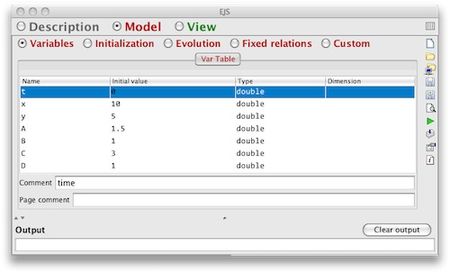
|style="width: 50%;|Step 2- we will create a simple visualization of the two populations versus time using EJS. After launching, we move to the Model portion of the interface. This is where we enter the variables for our simulation. Follow the directions and click to create a new page of variables. After giving the page a name, you add the variables described in the model. Variables are added by directly editing the variable table that was just created. | |style="width: 50%;|Step 2- we will create a simple visualization of the two populations versus time using EJS. After launching, we move to the Model portion of the interface. This is where we enter the variables for our simulation. Follow the directions and click to create a new page of variables. After giving the page a name, you add the variables described in the model. Variables are added by directly editing the variable table that was just created. | ||
|- | |- | ||
| − | |style="width: 50%;| | + | |style="width: 50%;|[[File:Easy_Java_Simulation_3_Evolution.jpg|450px]] |
| − | |style="width: 50%;| | + | |style="width: 50%;|[[File:Easy_Java_Simulation_4_Plotting_Frame.jpg|450px]] |
|- | |- | ||
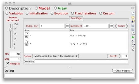
|style="width: 50%;|Step 3- The next step in creating our simulation is to describe how the model changes over time. Since we are using a differential equation model you need to move to the Evolution portion and create a page of ODEs. After naming the page, indicate the independent variable, t, and then enter the differential equations for the model. The equations can be inserted by double-clicking the table cells. | |style="width: 50%;|Step 3- The next step in creating our simulation is to describe how the model changes over time. Since we are using a differential equation model you need to move to the Evolution portion and create a page of ODEs. After naming the page, indicate the independent variable, t, and then enter the differential equations for the model. The equations can be inserted by double-clicking the table cells. | ||
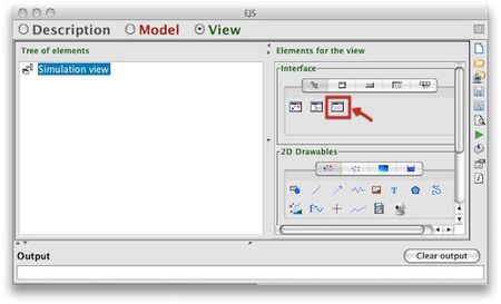
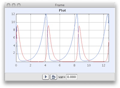
|style="width: 50%;|Step 4- Having defined the model, we move to the visualization. Our goal is to see how the predator and prey populations vary with time. Thus, we want to create a plot of x and y versus t. So, we add a plot to our visualization window. You accomplish this by clicking the PlottingFrame element highlighted below and then clicking Simulation View in the Tree of Elements. | |style="width: 50%;|Step 4- Having defined the model, we move to the visualization. Our goal is to see how the predator and prey populations vary with time. Thus, we want to create a plot of x and y versus t. So, we add a plot to our visualization window. You accomplish this by clicking the PlottingFrame element highlighted below and then clicking Simulation View in the Tree of Elements. | ||
|- | |- | ||
| − | |style="width: 50%;| | + | |style="width: 50%;|[[File:Easy_Java_Simulation_5_View.jpg|450px]] |
| − | |style="width: 50%;| | + | |style="width: 50%;|[[File:Easy_Java_Simulation_6_Finished_Example.jpg|450px]] |
|- | |- | ||
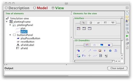
|style="width: 50%;|Step 5- we indicate what variables the plot will graph. By double clicking plot within the Tree of Elements, a new window pops up. Fill the Input X and Input Y fields with t and x respectively. To help differentiate the two populations, edit the Line Color parameter to be BLUE. Next we add a plot of the predator versus time by right-clicking the plot just edited and selecting Copy from the popup menu. Then right-click the plottingPanel element and select Paste. Edit the plot2 element so that Input Y is y. | |style="width: 50%;|Step 5- we indicate what variables the plot will graph. By double clicking plot within the Tree of Elements, a new window pops up. Fill the Input X and Input Y fields with t and x respectively. To help differentiate the two populations, edit the Line Color parameter to be BLUE. Next we add a plot of the predator versus time by right-clicking the plot just edited and selecting Copy from the popup menu. Then right-click the plottingPanel element and select Paste. Edit the plot2 element so that Input Y is y. | ||
Revision as of 12:04, 23 November 2016
Introduction
Easy Java Simulations is an open-source software tool, part of the Open Source Physics project, designed for the creation of discrete computer simulations.
In creating a simulation with the help of EJSS, the user does not program the simulation at the level of writing code, instead the user is working at a higher conceptual level, declaring and organizing the equations and other mathematical expressions that operate the simulation. EJSS handles the technical aspects of coding the simulation in the Java programming language, thus freeing the user to concentrate on the simulation's content.
Educational application and relevance
EJS is a software tool created to help science teachers and students with little or no programming background easily visualize scientific phenomena. Although the freeware application caters to scientific simulations, EJS can be applied to a wide variety of concepts. Simulations that result from programming with EJS can be quite complex, often masking the ease of the process involved in their creation.
Version
Current version EjsS_5.2_160712
Configuration
Overview of Features
EJS is a powerful tool that you may want to consider adopting for creating Java applications.
EJS can produce attractive simulations that allow user interaction.
EJS can produce quality simulations much more quickly than starting from scratch.
Other similar applications
not applicable
Development and community help
Working with the application
Functionalities
File formats for creation
EJSS has its own format for storing the simulations, which is based on XML, EJS and EJSS and carries the extension .xml, .ejs and .ejss. It contains not only the code for the simulation, but also the rest of the things, like the html introduction.
Saving the file
based on XML, EJS and EJSS and carries the extension .xml, .ejs and .ejss.
Export and publishing files
EjsS creates four subdirectories:
• config is the directory for user-defined configuration and options files.
• export is the proposed target directory when EjsS generates files for distribution.
• output is the directory used by EjsS to place temporary files generated when compiling a simulation.
• source is the directory under which all your simulation (source and auxiliary) files must be located.
Advanced features
Develop a prototype of an application in order to test an idea or algorithm.
Create user interfaces without programming.
Create models whose structure and algorithms non-programmers can inspect and understand.
Encourage students or colleagues (who may be new to Java) to create their own simulations.
Quickly prepare simulations to be distributed as applets or as stand alone programs.
Create a package containing multiple programs and the associated curricular material.
Installation
To install EjsS, do the following:
1. Install the Java Runtime Environment. EjsS requires the JavaRuntime Environment (JRE), version 1.7 or later. The JRE may already be installed in your computer, but, if not, visit the Java site.
2. Copy the EjsS distribution file to your computer. EjsS is distributed in a compressed ZIP file that can be downloaded from EjsS web site.
3. Uncompress EjsS. Uncompress the EjsS distribution file on your computer’s hard disk to create a directory called EJS X.x
And that’s it! This is all that is needed to install EjsS.
The application on mobiles and tablets
Currently there are no mobile and tablet applications for Easy Java Simulations.

