Learn LibreOffice Calc

Go back to
ICT student textbook
ICT teacher handbook

Introduction

The spreadsheet is a sheet with a collection of columns and rows. It contains number of cells. A cell is a combination or intersection of a row and a column, in which information both text and numeric can be input. A sheet can be simply understood as an array of cells. Altogether Spreadsheets are useful for capturing and analyzing data.

Basic information

ICT Competency	LibreOffice Calc is a free and open source application for creating generic resources. Spreadsheet is used for handling numeric data, analyzing and publishing through tables and graphs.
Educational application and relevance	Data analysis is an important mathematical competency. Spreadsheets can be very effective for introducing data analysis and statistics for students. It can also be used to explore patterns as an introduction to algebraic thinking. The power of the digital spreadsheet is that many types of data processing can be done on the information entered.
Version	Version: 7.3 (LibreOffice Calc is also available on the Windows and Macintosh operating systems)
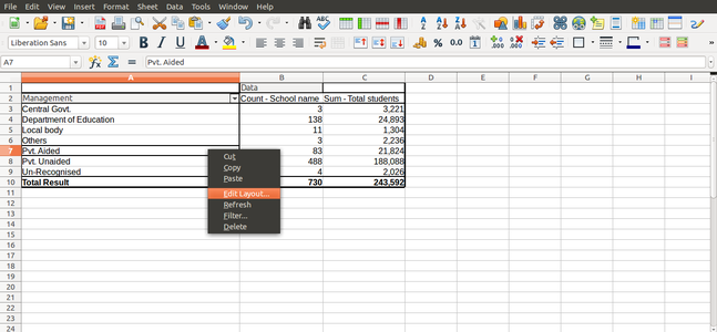
Configuration	No specific configuration requirements
Other similar applications	OnlyOffice, Collabora Office, Free Office
The application on mobiles and tablets	OnlyOffice for Android Collabora Office for Android and for iOS
Development and community help	Calc Manual Community help

Overview of features

Spreadsheet application is used for recording, processing and analyzing data. It is also used for creating text and graphical outputs. The application has many arithmetical, statistical, text processing functions which make it a very powerful desktop tool. Data can be sorted, filtered and processed into outputs, including multi-variate tables.

Installation

Please click on the below link to learn about LibreOffice Installation & Configuration

Click here

Working with the application

Download this file to practice on a simple sample data sheet.
Download this file of additional sheets with analyses, reports etc.

Opening a spreadsheet

Basic spreadsheet interface

LibreOffice Calc can be opened from "Applications --> Office --> LibreOffice Calc". This opens a ‘work book’. A work book can have many ‘sheets’. When you open the LO Calc application, it will show the window like as mentioned in the image above (Basic spreadsheet interface). The spreadsheet consists of rows and columns. Each column-row intersection is a cell; this is the place you will enter data in a spreadsheet. You can click the cursor on any cell and type in the information you want to enter.
Select Cell A1 and type “Name of city”, Hit enter. Next select cell B1 and type “Average annual rainfall (cms). Hit enter, and select cells of Column A to enter names of cities and Cells of Column B to enter annual average rainfall.
You can click on the A1 and B1 cells and click on the BOLD function icon (or simply type Ctrl+B) to make the headings bold.

Like in the case of text document, you can use the File menu to save your spreadsheet. The file will be saved with a .ods extension. ODS is the short form of Open Document Spreadsheet.

Navigating a spreadsheet

Navigation from various sheets

You can move across cells using the arrow keys. You can also quickly go to the ends of the sheet using "Ctrl" Key, such as Ctrl+Home (go to Cell A1), Ctrl+End (bottom rightmost part of filled cells / entered data), Ctrl + Up Arrow (next cell in same column, before an empty cell) etc.
It is useful to become comfortable using keyboard to move across the spreadsheet.
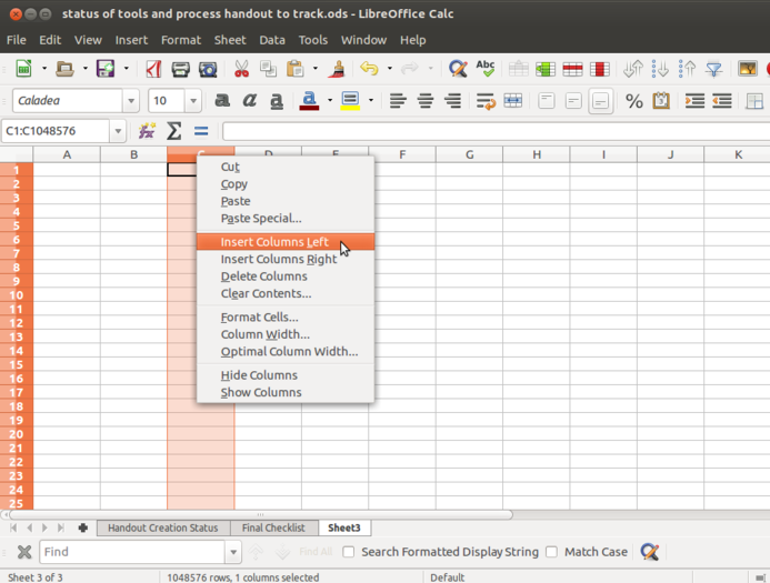
Columns and rows can be inserted or deleted or hidden in a spreadsheet. You can right click anywhere on the spreadsheet and insert/ delete rows and columns. You can also go to Sheet menu and insert rows/ columns.

Inserting a new sheet

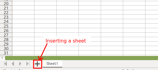
Inserting a new sheet
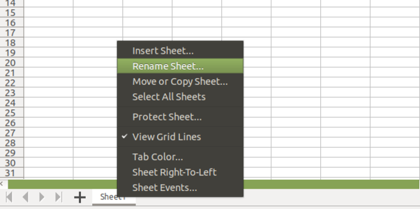
Renaming a sheet

Sheets can be added or deleted from a work book using the "+" symbol seen next to the sheet name. Sheets can be named and renamed by right clicking on the name of the sheet visible in the bottom panel.

Formatting a spreadsheet

Formatting in Calc

Formatting a spreadsheet involves two important formats.

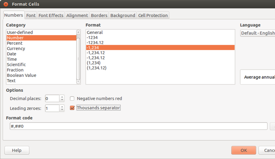
Text formatting : Text formatting involves making the text bold, italicized, increasing/reducing font size, font color etc. Data can also be formatted based on what it represents - date, time, currency, etc. The numeric information display format in terms of "000" separators or number of decimal places can be configured.

Alignment of Text inside the cell : Since Calc gives much importance for cells, the text alignment inside the cell also needs to be taken care of. Such alignments can be Top, center and bottom. Wrap text option allows the text which gone out of the cell to be aligned within the cell boundary.

There are two useful options associated with cells known as Merge cell and Split cell.

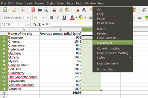
Merging the cell
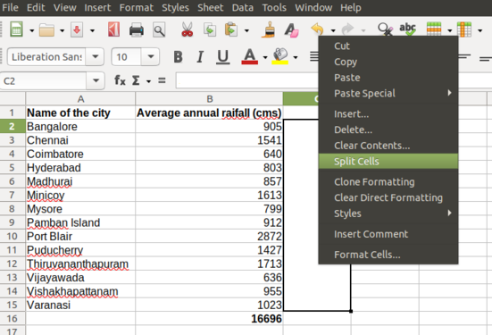
Splitting the cell

"Merge cell" combines two or more cells together to make it as one. For example, If you want the main heading to be given in a particular column which is having two or more sub menus or subsections you can use this feature.

To merge cells, select two or more cells and right click on anyone of the selected cells and click on "merge cell". For example, in the above image (Merging the cell) if you want to calculate the average rainfall of all the cities then you can merge the cells as shown in the image which indicates the calculated value is related to the entire column.

"Split cell" is needed when you accidentally merged the cells which are no longer required and you want them to be the separate cells.

To Split a merged cell, right click on the merged cell and click "split cell".

Freeze or Unfreeze rows and columns

If you enter data for a large number of rows or columns, you will not be able to read the row/column headings. To be able to see the column (and row) headings, you should move your cursor to the cell above which (and to the left of which) you want to be able to see your headings and click on "View --> Freeze Cells --> Freeze Rows and Columns".

Freezing the cells

Inserting formulae for computations

Inserting the formula

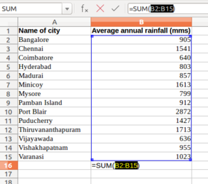
You can do almost any kind of computation or processing with a spreadsheet.

For example, here you can calculate the total rainfall for the cities. You can go to the cell below last row with data in Column B, which has the rainfall information and simply type in "=Sum(B2:B15)", assuming the data is in rows 2 through 15 of column B. Any computation or formula must begin with an "=" sign. Or you can simply use the shorthand icon on the menu bar “∑” where you will get various options like SUM, AVERAGE, MIN, MAX. Choose "SUM" here and hit "Enter" and the application will insert the same formula.

When the cursor is on this cell, the formula will be seen in the ‘formula’ bar on top of the sheet, below the menu.
All arithmetic operations, statistical operations are possible with spreadsheet.
You can ‘copy paste’ a formula from one cell to other cells in the same column, here ‘copy paste’ by default will copy paste the formula and not the content. This 'copy' and 'paste' of formula is not useful, when you want to 'fix' one value in our formula.
For instance, if you are computing 'Percentage of total' in the example of Average annual rainfall (cms) then, You can input in column C2 "=B2*100/B16". If you copy this cell C2 to C3, Calc will change the formula to "=B3*100/B17", since it will increment both numerator and denominator cells.
However consider you want to fix the denominator to 'B16'. To 'fix' the reference, you should insert '$' before the cell reference. So you should give formula C2 "=B2*100/B$16" since you want to fix the value in the 16th row. When you copy paste the formula to C3, it will copy as "=B3*100/B$16", which is what you want.

Sorting the data

Sorting the Data

You can sort the data in anyway you want. You could sort it on the descending order of the rainfall (Column B) to see the data by the cities with the heaviest rainfall at the top. You can sort the data by cities (Column B).

Note: You should select the entire sheet ("Edit --> Select All", or simply Ctrl+ A) or keep the cursor on a single cell, else you may sort only the data selected which will be incorrect.

Preparing charts and graphs

Selecting data for inserting charts
Selected Data Range
Renaming the Legend
Chart showing the annual rainfall

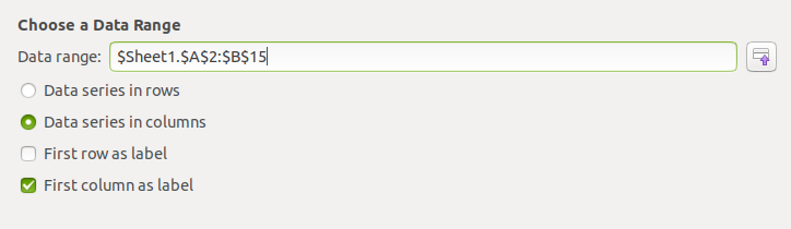
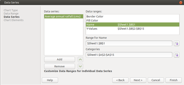
Select the data (columns A and B) and select "Insert --> Chart" option. You will get the chart wizard. You can select Bar chart to get a Bar chart of the rainfall. You should experiment with different graphical formats to learn about all the other charts.
Choose the Data Range. In this example it is A2 to B15.
Click on "Data series" column name on the left and on the right side modify the "Range for name" as done in the above image (Data Series image). At first it will show you the name of the column as "Column B". But if you want to modify it as the name of the column as mentioned in the spreadsheet then click on the "Name" in the "Data Ranges" table. Click on small icon which says "Select Data Range" --> A small window appears where you must click on the Column B1. Automatically it will consider the clicked column as the name for that field. Click "Next".
In the Last window Give the title if you want it to be appeared on the top of the chart. Click "Finish".

Working with Pivot tables

The pivot table (formerly known as Data Pilot) allows you to combine, compare, and analyze large amounts of data. You can view different summaries of the source data, you can display the details of areas of interest, and you can create reports. A table that has been created as a pivot table is an interactive table. Data can be arranged, rearranged or summarized according to different points of view.

Data sheet
Inserting Pivot

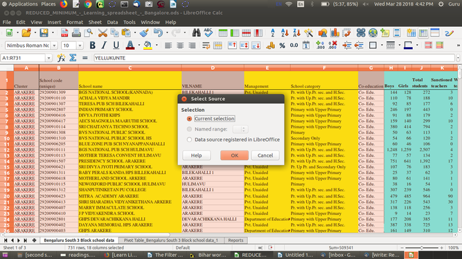
Position the cursor within a range of cells containing values, row and column headings.
Choose "Insert --> Pivot Table --> Create". The Select Source dialog appears. Choose Current selection and confirm with OK.
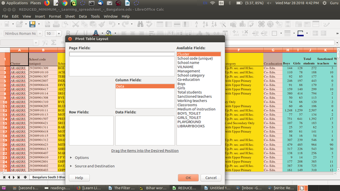
The table headings are shown as buttons in the Pivot Table dialog. Drag these buttons as required and drop them into the layout areas "Page Fields", "Column Fields", "Row Fields" and "Data Fields".
Drag the desired buttons into one of the four areas.

Selection wizard
Pivot Table wizard

Drag a button to the "Page Fields" area to create a button and a listbox on top of the generated pivot table. The listbox can be used to filter the pivot table by the contents of the selected item. You can use drag-and-drop within the generated pivot table to use another page field as a filter.

Insert data, row and column fields
Revising the data pivot for a new table

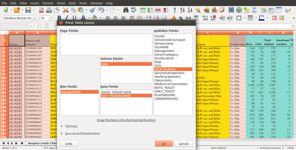
If the button is dropped in the "Data Fields" area it will be given a caption that also shows the formula that will be used to calculate the data.

By double-clicking on one of the fields in the "Data Fields" area you can call up the "Data Field" dialog.
Use the "Data Field" dialog to select the calculations to be used for the data. To make a multiple selection, press the "Ctrl" key while clicking the desired calculation.

Print Preview

Before printing any document you must make sure about the overall preview of the page. So get that you can click on "File--> Print Preview". This gives user the broader idea of how the printed material looks like.

Setting the margin

Click on margin icon for the flexible movement of margins in the spreadsheet.
Click on "Format Page" option to get various options such as "Page settings" to get the orientation of the page, Page borders to choose the style of the border, Inserting Header, Footer and other settings can be done.

In the image dotted lines represent the margins. They can be adjusted according to the printing needs.

Before printing the document go through these tips:

Use the "text wrap" feature to wrap all the text input in a cell so that it won’t overflow to the next cell.
Increase or reduce the column width so that all columns you want to print are included.
Delete (or hide) columns if you don’t want them in the printout.
Use "Format --> Page" option to insert header / footer information, such as file name, page number etc.
Use "Print preview" feature to keep checking if the formatting is satisfactory

Adding Page Header or Footer

Header/Footer option in Print Preview
Adding Header/Footer

Header or Footers make the document a neat presentation. Text added to the top of the margin is a Header. Text added to the bottom of the margin is a Footer. Header can include the name of the Book, Chapter name etc, whereas Footer may indicate the page number. In the "Print Preview" option, there will be a "Header and Footer" option as shown in the above image (Header/Footer option in Print Preview). Once clicked it gives you three areas where you can insert the Header, that is Left area, Center area and Right area. You can add the text at any area to apply it to all the pages. The same is applicable for Foote

Saving the files and formats

Like in most applications, a file can be saved using the File –-> Save command, or by the shortcut key Ctrl+S. Always give a meaningful file name, reading which you should get an idea of the file contents. This file has been named “Rainfall information for cities in South India, October 2016.ods”. Often adding the month-year information when the file was created can be useful later.
The files will be saved as ".ods". You can save a spreadsheet as a Microsoft Excel format also ("File --> Save As").
Main difference between "Save" and "Save As" is that Save Saves the document whereas Save As saves the document with another name.

The file you worked with can be exported to a PDF format. This is useful when you only need to print the file and do not want any changes to it. All the settings need to be done in the LibreOffice Calc and can be converted to PDF format.

Exporting the file to PDF

To do this, "File --> Export as PDF". A window appears which lets you to change the default settings. You can do the required changes and click "Export". In the next window it asks you to give the path where to export the file.

Advanced features

Calc is a very sophisticated software application and can even be used as a database, by cross referring data across sheets and books.
You can also generate multi-variate tables using the 'Pivot' feature.
The 'functions' in Calc are many and can meet statistical, logical, textual, mathematical functions which can be useful for exploring topics in Mathematics and Statistics.
You can use Calc to store contact information, which can be used along with the Thunderbird email client, to generate customized mass email messages (this functionality is called 'mail merge').
User defined formulae can be created and added to make the application more relatable.
You can repeat the column or row headings automatically across printed pages (hint – define print area). You can refer the references section for learning these advanced features.
Vlookup is an interesting feature with which you can query for a particular information using a simple syntax.

Ideas for resource creation

Calc can be used for analyzing data sets generated by your students as part of projects. Large secondary data sets can also be analyzed. Some of these project ideas include information about family members, houses in the area, crops / vegetation in the area, goods sold and prices in local shop and programs of the local government and budgets etc. The collected information can be analyzed and published in tabular cum graph formats.
Spreadsheets are also useful for helping solving numeric puzzles by setting up formulas and extrapolating.

References

Wikipedia
User manual for LO Calc
Community support
Videos to learn LO Calc are available in English, Telugu and other Indian languages on the Spoken-tutorials site, created by the NMEICT program of MHRD.