Difference between revisions of "Learn LibreOffice Calc"
| (One intermediate revision by the same user not shown) | |||
| Line 103: | Line 103: | ||
File:2. LO Calc Pivot 2. Inserting pivot.png|Inserting Pivot | File:2. LO Calc Pivot 2. Inserting pivot.png|Inserting Pivot | ||
</gallery> | </gallery> | ||
| − | + | 1. Position the cursor within a range of cells containing values, row and column headings. <br> | |
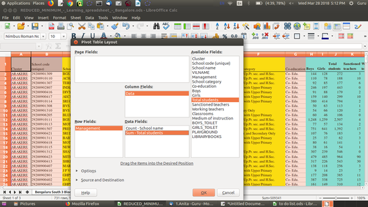
| − | + | 2. Choose Insert - Pivot Table - Create. The Select Source dialog appears. Choose Current selection and confirm with OK. The table headings are shown as <br> <gallery mode="packed" heights="280px" "caption="Adding the fields"> File:3. LO Calc Data Pivot 3. Current Selection.png|Selection wizard File:4. LO Calc Data Pivot 4. Pivot form.png|Pivot Table wizard </gallery> | |
| − | + | The table headings are shown as buttons in the Pivot Table dialog. Drag these buttons as required and drop them into the layout areas "Page Fields", "Column Fields", "Row Fields" and "Data Fields". <br> | |
| − | Drag a button to the '''Page Fields''' area to create a button and a listbox on top of the generated pivot table. The listbox can be used to filter the pivot table by the contents of the selected item. You can use drag-and-drop within the generated pivot table to use another page field as a filter. | + | 3. Drag the desired buttons into one of the four areas. <br> |
| + | Drag a button to the '''Page Fields''' area to create a button and a listbox on top of the generated pivot table. The listbox can be used to filter the pivot table by the contents of the selected item. You can use drag-and-drop within the generated pivot table to use another page field as a filter. <br> | ||
| − | If the button is dropped in the '''Data Fields''' area it will be given a caption that also shows the formula that will be used to calculate the data. | + | If the button is dropped in the '''Data Fields''' area it will be given a caption that also shows the formula that will be used to calculate the data. <br> |
* By double-clicking on one of the fields in the '''Data Fields''' area you can call up the [[Vnd.sun.star.help://scalc/text/scalc/01/12090105.xhp?Language=en-US&System=UNIX&UseDB=no&DbPAR=scalc|'''Data Field''']] dialog. | * By double-clicking on one of the fields in the '''Data Fields''' area you can call up the [[Vnd.sun.star.help://scalc/text/scalc/01/12090105.xhp?Language=en-US&System=UNIX&UseDB=no&DbPAR=scalc|'''Data Field''']] dialog. | ||
* Use the '''Data Field''' dialog to select the calculations to be used for the data. To make a multiple selection, press the Ctrl key while clicking the desired calculation. | * Use the '''Data Field''' dialog to select the calculations to be used for the data. To make a multiple selection, press the Ctrl key while clicking the desired calculation. | ||
Revision as of 12:32, 19 June 2018
IntroductionEarlier accountants used large pieces of paper to record business finances, to enter information like costs, payments, taxes, income etc. so that they got a complete financial overview. These large paper pieces were called “spreadsheets”. The digital spreadsheet is similar, with columns and rows. A cell is a combination or intersection of a row and a column, in which informationcaption="Working with Pivot tables" (both text and numeric) can be input. A sheet can be simply understood as an array of cells. 1.1 Basic information
Overview of featuresSpreadsheet application is used for recording data, processing data, analysing data, creating text and graphical outputs. The application has many statistical, arithmetical, text processing functions which makes it a very powerful desktop tool. Data can be sorted, filtered and processed into outputs, including multi-variate tables. Installation
Working with the application
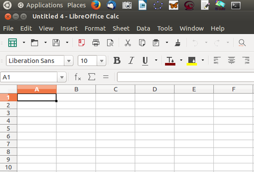
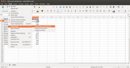
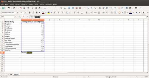
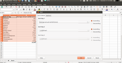
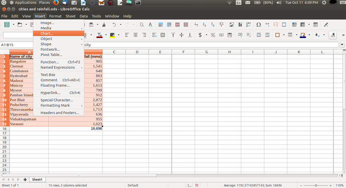
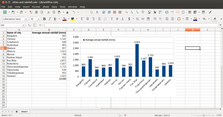
Opening a spreadsheetLibreOffice Calc can be opened from Applications → Office → LibreOffice Calc. This opens a ‘work book’. A work book can have many ‘sheets’. When you open the LO Calc application, it will show a window like this. The spreadsheet consists of rows and columns. Each column-row intersection is a cell; this is the place you will enter data in a spreadsheet. You can click the cursor on any cell and type in the information you want to enter. Like in the case of text document, you can use the File menu to save your spreadsheet. The file will be saved with a .ods extension. ODS is the short form of Open Document Spreadsheet. You can move across cells using the arrow keys. You can also quickly go to the ends of the sheet using CTRL Keys, such as CTRL-Home (go to Cell A1), CTRL-End (bottom rightmost part of filled cells / entered data), CTRL – Up Arrow (next cell in same column, before an empty cell) etc. Formatting a spreadsheetMost of the formatting options available in LibreOffice Writer are available in Calc also. Making the text bold, italicised, increasing/reducing font size, font color etc are all available. Data can also be formatted based on what it represents - date, time, currency, etc. The numeric information display format in terms of "000" separators or number of decimal places can be configured. Providing headings to the dataWe saw earlier how to enter headings for columns. However, if you enter data for more than 50 cities, you will not be able to read the column headings. To be able to see the column (and row) headings, you should move your cursor to the cell above which (and to the left of which) you want to be able to see your headings and click on View → Freeze Cells → Freeze Rows and Columns. Inserting formulae for computationsYou can do almost any kind of computation or processing with a spreadsheet. Here we will calculate the total rainfall for the cities. You can go to the cell below last row with data in Column B, which has the rainfall information and simply type in “=Sum(B2:B15)” assuming the data is in rows 2 through 15 of column B. Any computation or formula must begin with the “=” sign. Or you can simply use the shorthand icon on the menu bar “∑” and hit enter and the application will insert the same formula. Sorting the dataYou can sort the data in anyway you want. You could sort it on the descending order of the rainfall (Column B) to see the data by the cities with the heaviest rainfall at the top. You can sort the data by cities (Column B). remember that you should select the entire sheet (Edit – Select All, or simply CTRL-A) or keep the cursor on a single cell, else you may sort only the data selected which will be incorrect. Preparing charts and graphs
Working with Pivot tablesThe pivot table (formerly known as DataPilot) allows you to combine, compare, and analyze large amounts of data. You can view different summaries of the source data, you can display the details of areas of interest, and you can create reports. A table that has been created as a pivot table is an interactive table. Data can be arranged, rearranged or summarized according to different points of view.
1. Position the cursor within a range of cells containing values, row and column headings. The table headings are shown as buttons in the Pivot Table dialog. Drag these buttons as required and drop them into the layout areas "Page Fields", "Column Fields", "Row Fields" and "Data Fields". If the button is dropped in the Data Fields area it will be given a caption that also shows the formula that will be used to calculate the data.
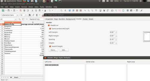
Printing a spreadsheetFormatting a sheet for printing is not an easy task. To make it simpler, some tips are:
Saving the files and formats
Advanced featuresCalc is a very sophisticated software application and can even be used as a database, by cross referring data across sheets and books. You can also generate multi-variate tables using the 'Pivot' feature. The 'functions' in Calc are many and can meet statistical, mathematical functions which can be useful for exploring topics in Mathematics and Statistics. You can use Calc to store contact information, which can be used along with the Thunderbird email client, to generate customised mass email messages (this functionality is called 'mail merge'). You can repeat the column or row headings automatically across printed pages (hint – define print area). You can refer to the Calc user manual for learning these advanced features Ideas for resource creation
References
|

